Start here: 2×2 square with axial load
| Author: | Nicolás Guarín-Zapata |
|---|---|
| Date: | May, 2017 |
In this document we briefly describe the use of SolidsPy, through a simple example corresponding to a square plate under point loads.
Input files
The code requires the domain to be input in the form of text files
containing the nodes, elements, loads and material information. These
files must reside in the same directory and must have the names
eles.txt, nodes.txt, mater.txt and loads.txt. Assume
that we want to find the response of the 2×2 square under unitary
vertical point loads shown in the following figure. Where one corner is
located at (0,0) and the opposite one at (2,2).
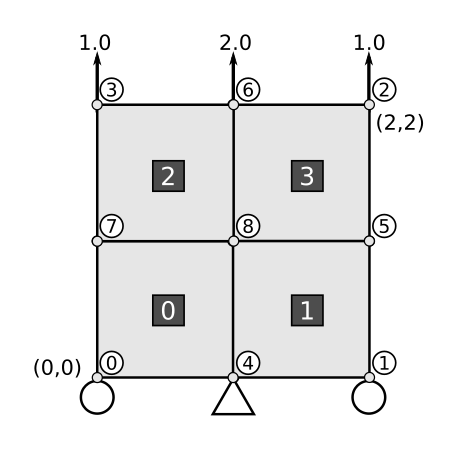
4-element solid under point loads.
The file nodes.txt is composed of the following fields:
- Column 0: Nodal identifier (integer).
- Column 1: x-coordinate (float).
- Column 2: y-coordinate (float).
- Column 3: Boundary condition flag along the x-direction (0 free, -1 restrained).
- Column 4: Boundary condition flag along the y-direction (0 free, -1 restrained).
The corresponding file has the following data
0  0.00  0.00   0  -1
1  2.00  0.00   0  -1
2  2.00  2.00   0   0
3  0.00  2.00   0   0
4  1.00  0.00  -1  -1
5  2.00  1.00   0   0
6  1.00  2.00   0   0
7  0.00  1.00   0   0
8  1.00  1.00   0   0
The file eles.txt contain the element information. Each line in the
file defines the information for a single element and is composed of the
following fields:
- Column 0: Element identifier (integer).
- Column 1: Element type (integer):
- 1 for a 4-noded quadrilateral.
- 2 for a 6-noded triangle.
- 3 for a 3-noded triangle.
- Column 2: Material profile for the current element (integer).
- Column 3 to end: Element connectivity, this is a list of the nodes conforming each element. The nodes should be listed in counterclockwise orientation.
The corresponding file has the following data
0   1   0   0   4   8   7
1   1   0   4   1   5   8
2   1   0   7   8   6   3
3   1   0   8   5   2   6
The file mater.txt contain the material information. Each line in
the file corresponds to a material profile to be assigned to the
different elements in the elements file. In this example, there is one
material profile. Each line in the file is composed of the following
fields:
- Column 0: Young’s modulus for the current profile (float).
- Column 1: Poisson’s ratio for the current profile (float).
The corresponding file has the following data
1.0 0.3
The file loads.txt contains the point loads information. Each line
in the file defines the load information for a single node and is
composed of the following fields
- Column 0: Nodal identifier (integer).
- Column 1: Load magnitude for the current node along the x-direction (float).
- Column 2: Load magnitude for the current node along the y-direction (float).
The corresponding file has the following data
3  0.0  1.0
6  0.0  2.0
2  0.0  1.0
Executing the program
After installing the package, you can run the program in a Python terminal using
>>> from solidspy import solids_GUI
>>> solids_GUI()
In Linux and you can also run the program from the terminal using
$ python -m solidspy
If you have easygui installed a pop-up window will appear for you to
select the folder with the input files
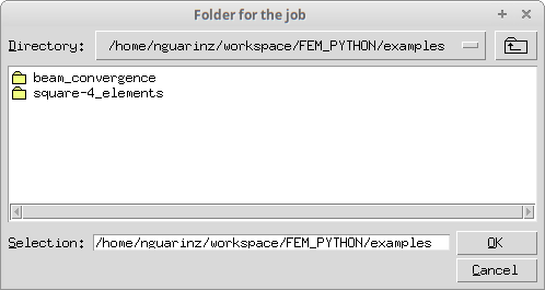
Folder selection window.
select the folder and click ok.
If you don’t have easygui installed the software will ask you for
the path to your folder. The path can be absolute or relative.
Enter folder (empty for the current one):
Then, you will see some information regarding your analysis
Number of nodes: 9
Number of elements: 4
Number of equations: 14
Duration for system solution: 0:00:00.006895
Duration for post processing: 0:00:01.466066
Analysis terminated successfully!
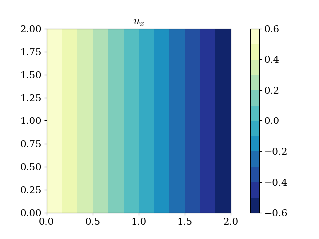
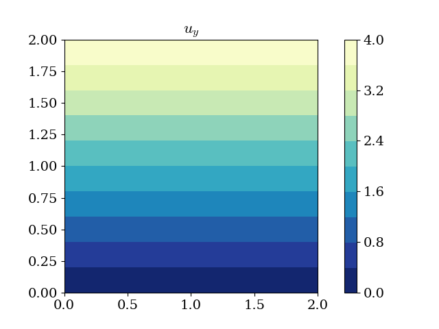
And, once the solution is achieved you will see displacements and stress solutions as contour plots, like the following
Interactive execution
You can also run the program interactively using a Python terminal, a good option is IPython.
In IPython you can run the program with
In [1]: from solidspy import solids_GUI

In [2]: UC = solids_GUI()
After running the code we have the nodal variables for post-processing. For example, we can print the displacement vector
In [3]: np.set_printoptions(threshold=np.nan)

In [4]: print(np.round(UC, 3))
[ 0.6 -0.6 -0.6  4.   0.6  4.  -0.6  2.  -0.   4.   0.6  2.  -0.   2. ]
where we first setup the printing option for IPython to show the full array and then rounded the array to 3 decimal places.
In [5]: U_mag = np.sqrt(UC[0::2]**2 + UG[1::2]**2)

In [6]: print(np.round(U_mag, 3))
[ 0.849  4.045  4.045  2.088  4.     2.088  2.   ]