Geometry in Gmsh and solution with SolidsPy
| Author: | Nicolás Guarín-Zapata |
|---|---|
| Date: | September, 2018 |
This document is a tutorial on how to generate a (specific) geometry using Gmsh [Gmsh2009] and its subsequent processing for the generation of input files for a Finite Element program in Python. This document does not pretend to be an introduction to the management of Gmsh, for this we suggest the official tutorial [Gmsh_tut] (for text mode) or the official screencasts [Gmsh_scr] (for the graphical interface).
Model
The example to be solved corresponds to the determination of Efforts in a cylinder in the Brazilian Test. The Brazilian Test is a technique that is used for the indirect measurement of the resistance of rocks It is a simple and effective technique, and therefore it is commonly used for rock measurements. Sometimes this test is also used for concrete [D3967-16].
The following figure presents a scheme of the model to solve. Since the original model may present rigid body movements, it decides to use the symmetry of the problem. Then, the problem to solve is a quarter of the original problem and the surfaces lower e left present restrictions of roller.

Schematic of the problem to be solved.
Creation of the geometry and mesh in Gmsh
As a first step, it is suggested to create a new file in Gmsh, as It shows in the following figure.
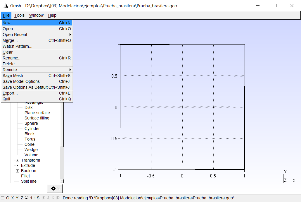
Creation of a new file in Gmsh.
When creating a new document it is possible [1] for Gmsh to ask about which
geometry kernel to use. We will not dwell on what the differences are
and we will use built-in.

Pop-up window asking for the geometry kernel.
To create a model, we initially create the points. For that, let’s go
to the option: Geometry> Elementary Entities> Add> Point, as
shown in the following figure. Then, the coordinates of the
points in the pop-up window and “Add”. Finally we can close the
pop-up window and press e.
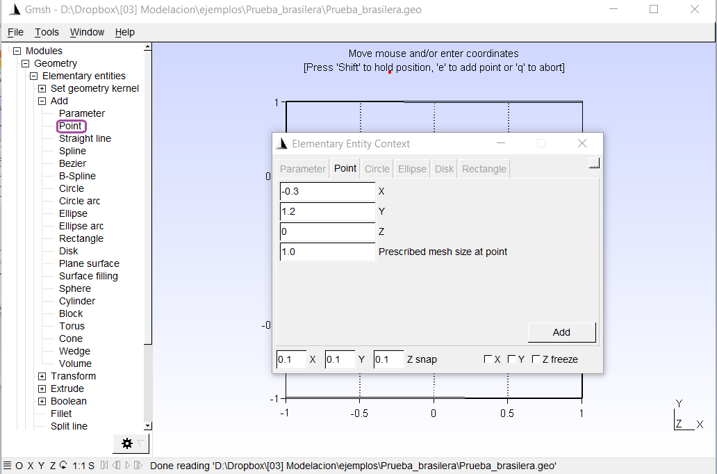
Agregar puntos al modelo.
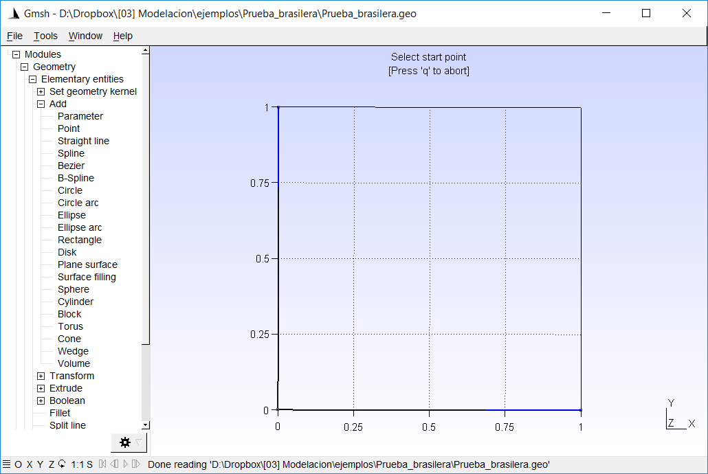
Later we create lines. For this, we go to the option:
`` Geometry> Elementary Entities> Add> Straight line``, as
shown in the following figure, and we select the initial points and
endings for each line. At the end, we can press e.
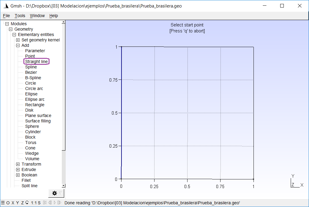
Add straight lines to the model.
We also create the circle arcs. For this, we go to the
option: Geometry> Elementary Entities> Add> Circle Arc, as
shown in the following figure, and we select the initial points,
central and final for each arc (in that order). At the end, we can
press e.
Add arcs to the model.
Since we already have a closed contour, we can define a surface.
For this, we go to the option:
Geometry> Elementary Entities> Add> Plane Surface, as
shown in the following figure, and we select the contours in order.
At the end, we can press `` e``.
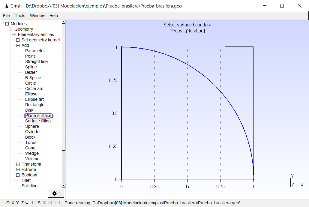
Add surfaces.
Now, we need to define physical groups. Physical groups allow us to associate names to different parts of the model such as lines and surfaces. This will allow us to define the region in which we will resolve the model (and we will associate a material), the regions that have restricted movements (boundary conditions) and the regions on which we will apply the load. In our case we will have 4 groups physical:
- Region of the model, where we will define a material;
- Bottom edge, where we will restrict the displacement in \(y\);
- Left edge, where we will restrict the displacement in \(x\); and
- Top point, where we will apply the point load.
To define the physical groups we are going to
Geometry> Physical groups> Add> Plane Surface, as shown in the
next figure. In this case, we can leave the field of `` Name`` empty
and allow Gmsh to name the groups for us, which will be
numbers that we can then consult in the text file
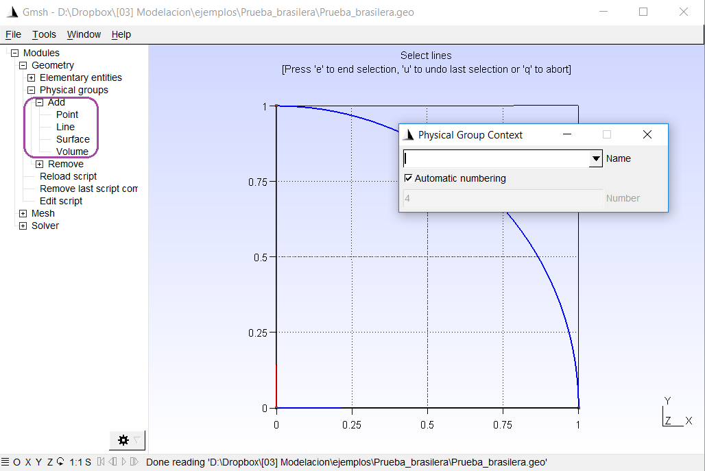
Add physical groups.
After (slightly) editing the text file (.geo) this looks like this
L = 0.1;

// Points
Point(1) = {0, 0, 0, L};
Point(2) = {1, 0, 0, L};
Point(3) = {0, 1, 0, L};

// Lines
Line(1) = {3, 1};
Line(2) = {1, 2};
Circle(3) = {2, 1, 3};

// Surfaces
Line Loop(1) = {2, 3, 1};
Plane Surface(1) = {1};

// Physical groups
Physical Line(1) = {1};
Physical Line(2) = {2};
Physical Point(3) = {3};
Physical Surface(4) = {1};
We added a parameter L, which we can vary to
to change the size of the elements when creating the
mesh.
Now, we proceed to create the mesh. To do this, we go to Mesh> 2D.
As we see in the figure below.
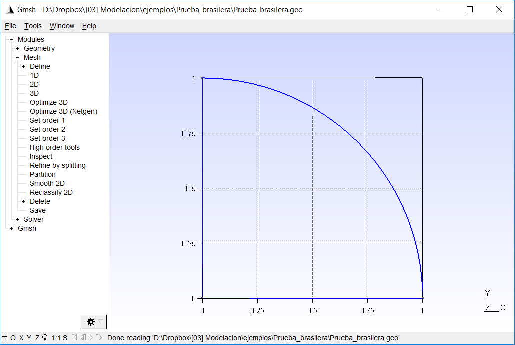
Create the mesh.
Additionally, we can change the configuration so that it shows the elements
of the mesh in colors. For this, we are going to
Tools> Options> Mesh and mark the box that indicates
Surface faces.
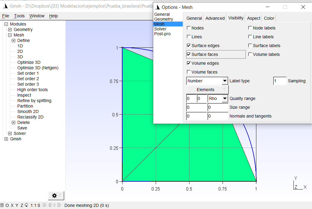
Create the mesh.
We can then refine the mesh going to
Mesh> Refine by Splitting, or by modifying the L parameter in the
input file (.geo). As a last step, we want to save the mesh.
To do this, go to Mesh> Save, or File> Save Mesh, as
shows below.
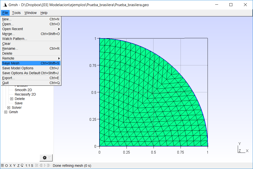
Save the .msh file.
Python script to generate input files
We need to create files with the information of the nodes (nodes.txt),
elements (eles.txt), loads (loads.txt) and materials
(mater.txt).
The following code generates the necessary input files for Run the finite element program in Python.
import meshio
import numpy as np

mesh = meshio.read("Prueba_brasilera.msh")
points = mesh.points
cells = mesh.cells
point_data = mesh.point_data
cell_data = mesh.cell_data

# Element data
eles = cells["triangle"]
els_array = np.zeros([eles.shape[0], 6], dtype=int)
els_array[:, 0] = range(eles.shape[0])
els_array[:, 1] = 3
els_array[:, 3::] = eles

# Nodes
nodes_array = np.zeros([points.shape[0], 5])
nodes_array[:, 0] = range(points.shape[0])
nodes_array[:, 1:3] = points[:, :2]

# Boundaries
lines = cells["line"]
bounds = cell_data["line"]["gmsh:physical"]
nbounds = len(bounds)

# Loads
id_cargas = cells["vertex"]
nloads = len(id_cargas)
load = -10e8 # N/m
loads_array = np.zeros((nloads, 3))
loads_array[:, 0] = id_cargas
loads_array[:, 1] = 0
loads_array[:, 2] = load

# Boundary conditions
id_izq = [cont for cont in range(nbounds) if bounds[cont] == 1]
id_inf = [cont for cont in range(nbounds) if bounds[cont] == 2]
nodes_izq = lines[id_izq]
nodes_izq = nodes_izq.flatten()
nodes_inf = lines[id_inf]
nodes_inf = nodes_inf.flatten()
nodes_array[nodes_izq, 3] = -1
nodes_array[nodes_inf, 4] = -1

#  Materials
mater_array = np.array([[70e9, 0.35],
                        [70e9, 0.35]])
maters = cell_data["triangle"]["gmsh:physical"]
els_array[:, 2]  = [1 for mater in maters if mater == 4]

# Create files
np.savetxt("eles.txt", els_array, fmt="%d")
np.savetxt("nodes.txt", nodes_array,
           fmt=("%d", "%.4f", "%.4f", "%d", "%d"))
np.savetxt("loads.txt", loads_array, fmt=("%d", "%.6f", "%.6f"))
np.savetxt("mater.txt", mater_array, fmt="%.6f")
Now, let’s discuss the different parts of the code to see what it does each.
Header and reading the .msh file
The first part loads the necessary Python modules and reads the file
of mesh that in this case is called Prueba_brasilera.msh (line 6 and
7). In order for Python to be able to read the file, it must be in the
same directory as the Python file that will process it.
import meshio
import numpy as np


mesh = meshio.read("Prueba_brasilera.msh")
points = mesh.points
cells = mesh.cells
point_data = mesh.point_data
cell_data = mesh.cell_data
Element data
The next section of the code creates the data for elements. The line
18 creates a variable `` eles`` with the information of the nodes that
make up each triangle. Line 11 creates an array (filled with zeros)
with the number of rows equal to the number of elements
(eles.shape[0]) and 6 columns [2]. Then we assign a number to
each element, what we do on line 12 with range(eles.shape[0])
and this we assign to column 0. All
elements are triangles, that’s why we should put 3 in column 1. Last,
in this section, we assign the nodes of each element to the array
with (line 19), and this assignment is made from column 3 to
final with els_array[:, 3::].
# Element data
eles = cells["triangle"]
els_array = np.zeros([eles.shape[0], 6], dtype=int)
els_array[:, 0] = range(eles.shape[0])
els_array[:, 1] = 3
els_array[:, 3::] = eles
Nodes data
In the next section we create the information related to the
nodes. To do this, on line 17 we created an array nodes_array
with 5 columns and as many rows as there are points in the model
(points.shape[0]). Then, we assign the
element type on line 18. And finally, we assign the
information on the coordinates of the nodes on line 19 with
nodes_array[:, 1:3] = points[:, :2], where we are adding the
information in columns 1 and 2.
# Nodes
nodes_array = np.zeros([points.shape[0], 5])
nodes_array[:, 0] = range(points.shape[0])
nodes_array[:, 1:3] = points[:, :2]
Boundary data
In the next section we find the line information. For this,
we read the cells information in position line [3]
(line 22). The array lines
will then have the information of the nodes that form each
line that is on the border of the model. Then, we read the information
of the physical lines (line 23), and we calculate how many lines belong
to the physical lines (line 24).
# Boundaries
lines = cells["line"]
bounds = cell_data["line"]["gmsh:physical"]
nbounds = len(bounds)
Load data
In the next section we must define the information of loads.
In this case, the loads are assigned in a single point that we define as a
physical group. On line 27 we read the nodes (in this case, one).
Then, we create an array that has as many rows as loads (nloads) and 3
columns Assign the number of the node to which each load belongs
(line 31), the charges in :math: x (line 32) and the loads in \(y\) and
(line 33)
# Loads
id_cargas = cells["vertex"]
nloads = len(id_cargas)
load = -10e8 # N/m
loads_array = np.zeros((nloads, 3))
loads_array[:, 0] = id_cargas
loads_array[:, 1] = 0
loads_array[:, 2] = load
Boundary conditions
Now, we will proceed to apply the boundary conditions, that is, the model regions that have restrictions on displacements. Initially, we identify which lines have an identifier 1 (which would be the left side) with
id_izq = [cont for cont in range(nbounds) if bounds[cont] == 1]
This creates a list with the numbers (cont) for which the
condition (bounds[cont] == 1). On line 46 we get the nodes that belong to
these lines, however, this array has as many rows as lines
on the left side and two columns. First we return this array as
a one-dimensional array with nodes_izq.flatten(). Later, on line 42,
we assign the value of -1 in the third column of the array for
nodes that belong to the left side. In the same way, this process
is repeated for the nodes at the bottom line.
# Boundary conditions
id_izq = [cont for cont in range(nbounds) if bounds[cont] == 1]
id_inf = [cont for cont in range(nbounds) if bounds[cont] == 2]
nodes_izq = lines[id_izq]
nodes_izq = nodes_izq.flatten()
nodes_inf = lines[id_inf]
nodes_inf = nodes_inf.flatten()
nodes_array[nodes_izq, 3] = -1
nodes_array[nodes_inf, 4] = -1
Materials
In the next section we assign the corresponding materials to each
element. In this case, we only have one material. However, it
present the example as if there were two different ones. First, we created a
array with the material information where the first column
represents the Young’s module and the second the Poisson’s relation (line
46). Then, we read the information of the physical groups of surfaces
on line 48. Finally, we assign the value of 0 to the materials that
have as physical group 4 (see file .geo above) and 1 to the
others, which in this case will be zero (line 49). This information goes in the
column 2 of the arrangement.
#  Materials
mater_array = np.array([[70e9, 0.35],
                        [70e9, 0.35]])
maters = cell_data["triangle"]["gmsh:physical"]
els_array[:, 2]  = [1 for mater in maters if mater == 4]
Export files
The last section uses the numpy function to export the
files.
# Create files
np.savetxt("eles.txt", els_array, fmt="%d")
np.savetxt("nodes.txt", nodes_array,
         fmt=("%d", "%.4f", "%.4f", "%d", "%d"))
np.savetxt("loads.txt", loads_array, fmt=("%d", "%.6f", "%.6f"))
np.savetxt("mater.txt", mater_array, fmt="%.6f")
Solution using SolidsPy
To solve the model, we can type [4]
from solidspy import solids_GUI
disp = solids_GUI()
After running this program it will appear a pop-up window as shown below. In this window the directory we should locate the folder with the input files generated previously. Keep in mind that the appearance of this window may vary between operating systems. Also, we have notef that sometimes the pop-up window may be hidden by other windows on your desktop.
Pop-up window to locate folder with input files.
At this point, the program must solve the model. If the input files are used without modifications the program should print a message similar to the following.
Number of nodes: 123
Number of elements: 208
Number of equations: 224
Duration for system solution: 0:00:00.086983
Duration for post processing: 0:00:00
Analysis terminated successfully!
the times taken to solve the system can change a bit from one computer to another.
As a last step, the program generates graphics with the fields of displacements, deformations and stresses, as shown in the next figures.

Horizontal displacement.

Vertical displacement.
References
| [D3967-16] | ASTM D3967–16 (2016), Standard Test Method for Splitting Tensile Strength of Intact Rock Core Specimens, ASTM International, www.astm.org. |
| [Gmsh2009] | Geuzaine, Christophe, y Jean-François Remacle (2009), Gmsh: A 3-D finite element mesh generator with built-in pre-and post-processing facilities. International Journal for Numerical Methods in Engineering, 79.11. |
| [Gmsh_tut] | Geuzaine, Christophe, y Jean-François Remacle (2017), Gmsh Official Tutorial. Accessed: April 18, 2018 http://gmsh.info/doc/texinfo/gmsh.html#Tutorial. |
| [Gmsh_scr] | Geuzaine, Christophe, y Jean-François Remacle (2017), Gmsh Official Screencasts. Accessed: April 18, 2018de http://gmsh.info/screencasts/. |
| [1] | If the version is 3.0 or higher, this pop-up window will appear. |
| [2] | For quadrilateral elements, 7 columns would be used, since each Element is defined by 4 nodes. |
| [3] | cells is a dictionary and allows to store information associated
with some keywords, in this case it is lines. |
| [4] | To make use of the graphical interface it must be installed
easygui. |